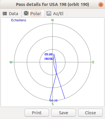
Another satellite newbie question from my side. I have troubles understanding SDS-3 F-5’s polar plots as shown in the following scheduled observation’s polar plot: https://network.satnogs.org/observations/3013754/
(all other plots of SDS-3 F-5 over my station show similar behavior)
If i understand correctly SDS-3 F-5 has a highly elliptical orbit (with most time over the northern hemisphere) which could explain some ‘strange’ ground tracks including ‘loops’. But there should still some kind of pass over the horizon. The SatNOGS polar plot of a pass show most of the pass below the horizon. Is there some anomaly in the way the polar plots are plotted or is this inherently something related to highly elliptical orbits ?
These highly elliptical orbits are called Molniya orbits. These orbits have several properties.
They are aimed for an orbital period of half a day, such that the ground track of the orbit repeats after every second orbit.
They use an inclination of 63.4 degrees, such that the precession of the point of perigee due to the oblateness of the Earth is zero, meaning that the point where perigee is in their orbit does not drift with time.
They use an eccentric orbit to maximize the dwell time over certain latitudes. Most satellites in Molniya orbit provide services to the Northern hemisphere, so apogee is over the Northern hemisphere. This needs an argument of perigee of 270 degrees.
Molniya orbits are heavily used by Russia to provide communications over the Northern hemisphere, as geostationary orbits are less useful at the Northernmost latitudes. By placing three satellites in the same orbital plane, separated by 120 degrees, you can guarantee one of them will be in view at any time.
I agree that the plot looks odd. We probably need to check that code that it also deals with eccentric orbits.
Note that SatNOGS will likely fail trying to observe these satellites. As their passes take hours, it is likely that you’ll fill up the Raspberry Pi before the end of the pass.
Used GPredict to plot the same sat and the plots look like what i expect from your explanations, 2 different ground tracks that repeat every day:
Same location used as for my ground station, as i didn’t manage to import the TLE from SatNOGS into GPredict, the one fetched from tleupdate has been used.
Yes the observations are really long and it would be nice to be able to select only a limited timeframe out of it for an observation. As my s-band tests are done in a docker on my computer i’m currently not limited to the space of a raspberry.
Got an almost 3 hours observation here: SatNOGS Network - Observation 3003400
There is something like a thin vertical trace that could be a carrier, but the orientation of the background noise seems strange.
Another observation of ‘the other pass’ during which the satellite didn’t seem to move: SatNOGS Network - Observation 2717696
The same thin lines appears better (antenna is better orientated for it), this time the background noise doesn’t appear slatted as no/only minimal doppler correction.
On short timescales the velocity change for these HEO satellites is very small. Your best bet to get the best chance of detection is near the beginning and end of a pass when the satellite is moving towards or away from perigee. Here, the velocity changes are largest, though the satellite is also lowest on the horizon.
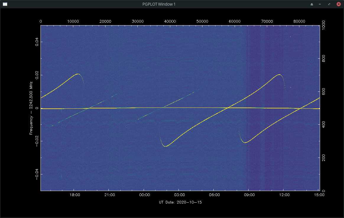
Here is a plot of 2242.5MHz for a day long scan using an 3.5 turn helical antenna, capturing and plotting the data with strf.
It shows the Doppler curves of two SDS satellites in a Molniya orbit (the diagonal curves), as well as one of the SDS satellites in GEO (the horizontal curve). The hooks at the start and end of two of the HEO curves are when it rises or sets over the Southern horizon. The two curves without the hooks are when it is visible low over the Northern horizon.
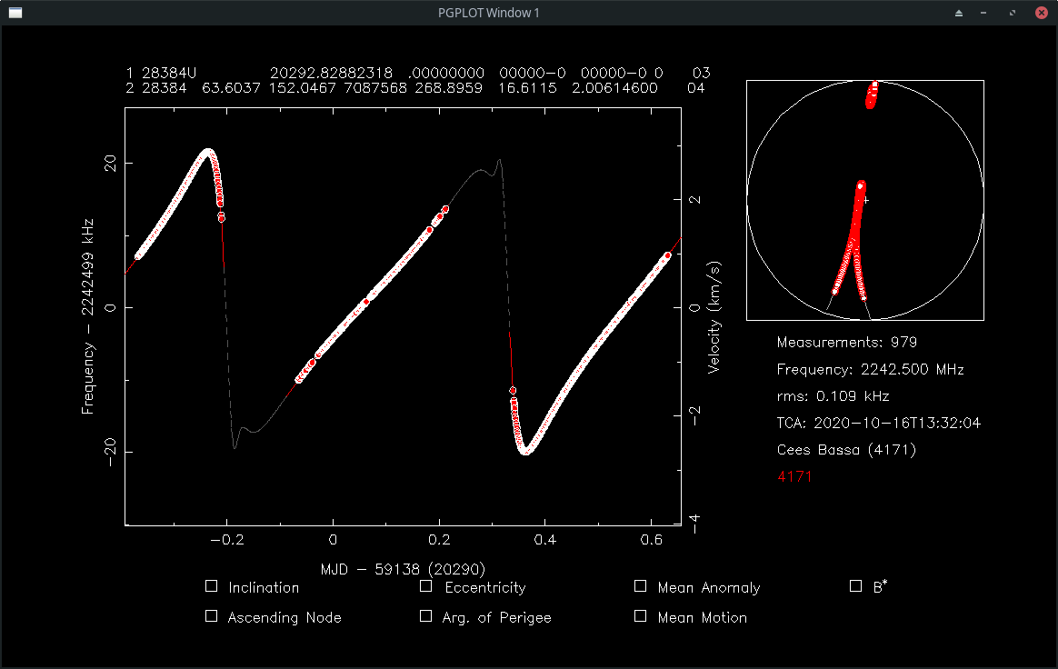
Here is a plot of the extracted Doppler curve for one of the two HEO SDS satellites (USA 179 [28384/04034A]) compared to a prediction from a TLE. The red parts of the predicted curve are above my horizon, the grey parts below. The polar plot on the top left shows the track on the sky.
Detecting the narrowband signal with the SatNOGS setup may be difficult, as the integration time in the waterfall is quite short and the channels are narrow. With STRF I integrate for 1 second and use 100Hz channels in the top plot.
Thanks for these detailed explanations @cgbsat, there is still so much to learn. Looking forward to have time to build my VLNA13 so hopefully this will give me better signals to do more observations.